3 Observational Studies
Class materials
Slides: Module 3
Interactive: Sensitivity Analysis Explorer
Textbook reading
Supplementary reading
Rosenbaum PR. (2002). Observational Studies. 2nd ed. Springer. VanderWeele TJ, Ding P. (2017). Sensitivity Analysis in Observational Research: Introducing the E-Value. Annals of Internal Medicine, 167(4), 268–274.
Topics covered
- The challenge of confounding in public health and medical research
- From Bradford Hill’s criteria to modern causal inference
- Exchangeability, positivity, and consistency (SUTVA)
- Effect identification in observational studies
- Checklist Item 4: Could confounding explain the result?
- Critical reading exercise: evaluating the Framingham Heart Study
3.1 The challenge of confounding in public health and medical research
Confounding is a major challenge in public health and medical research because it can create misleading associations between exposures and outcomes. A confounder is a third variable that is associated with both the exposure and the outcome, potentially distorting the true causal relationship. For example, if we observe that people who carry lighters tend to have higher rates of lung cancer, we might wrongly conclude that carrying a lighter causes cancer. In reality, smoking is the confounding variable: smokers are more likely to carry lighters and also more likely to develop lung cancer. Without properly adjusting for confounders, studies risk producing biased estimates, leading to incorrect conclusions about risk factors, treatments, or interventions.
Addressing confounding is crucial but not always straightforward. Methods such as stratification, multivariable regression, propensity score matching, and inverse probability weighting are commonly used to try to adjust for or eliminate confounding effects. However, identifying all relevant confounders can be difficult, especially when dealing with observational data where randomization is not possible. Unmeasured or unknown confounders remain a constant threat to validity. Therefore, careful study design, domain knowledge, and sensitivity analyses are essential to minimize the impact of confounding and ensure more reliable and actionable public health research findings.
Example Setup Let’s say we want to study the effect of Exercise (X) on Heart Health (Y), but there’s a Genetic Factor (Z) that causes both Exercise and Heart Health. In this case, Z is a confounder, and we should adjust for it.
In this simulation we will have two models: a naive model and an adjusted model. The naive model will only regress heart health on exercise. The adjusted model will regress heart health on exercise and genetic factors, which controls for genetic factor being a confounder. Since this is a simulated example, we know that the true effect of exercise on heart health is 0.8. We will see in this example that the estimated causal effect coming from the adjusted model is better than the naive model.
n <- 2000
genetics <- rnorm(n)
exercise <- 0.6 * genetics + rnorm(n)
heart_health <- 0.8 * exercise + 0.5 * genetics + rnorm(n)
df <- data.frame(heart_health, exercise, genetics)
model_naive <- lm(heart_health ~ exercise, data = df)
summary(model_naive)$coefficients["exercise", ]
## Estimate Std. Error t value Pr(>|t|)
## 1.018337 0.020338 50.070657 0.000000model_adjusted <- lm(heart_health ~ exercise + genetics, data = df)
summary(model_adjusted)$coefficients["exercise", ]## Estimate Std. Error t value Pr(>|t|)
## 8.080949e-01 2.126973e-02 3.799272e+01 3.610292e-238# library(ggplot2)
naive_estimate <- summary(model_naive)$coefficients["exercise", "Estimate"]
adjusted_estimate <- summary(model_adjusted)$coefficients["exercise", "Estimate"]
estimates <- data.frame(
Model = c("Naive", "Adjusted"),
Estimate = c(naive_estimate, adjusted_estimate)
)
ggplot(estimates, aes(x = Model, y = Estimate, fill = Model)) +
geom_col(width = 0.5) +
labs(title = "Comparison of Naive vs Adjusted Estimates",
y = "Estimated Effect of Exercise",
x = "") +
geom_hline(yintercept = 0.8, linetype = 2) +
annotate("text", x = 2.45, y = 0.85, label = "True effect") +
theme_minimal() +
theme(legend.position = "none")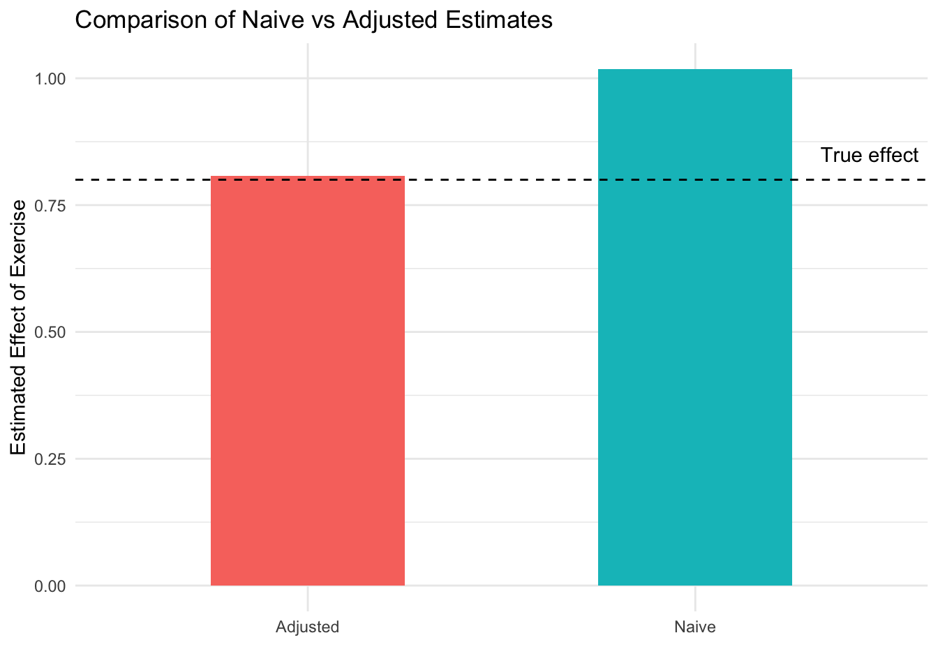
In this simulation, we model a situation where Genetics (Z) is a confounder that influences both Exercise (X) and Heart Health (Y). The naive model, which regresses Heart Health on Exercise without adjusting for Genetics, gives a biased estimate of the effect of Exercise (1.05). This happens because part of the observed association is actually due to Genetics, not Exercise itself. When we adjust for Genetics in the second model, the estimate of Exercise’s effect (0.84) becomes more accurate, isolating its true relationship with Heart Health. This is shown in how the bar for the adjusted graph is closer to the dotted black line, which represents the true causal effect of exercise (0.8). This example highlights how failing to account for confounding can lead researchers to overstate or misinterpret causal effects in public health and medical studies.
3.2 From Bradford Hill’s criteria to modern causal inference
Before the formal tools of modern causal inference existed, researchers needed a framework for evaluating whether an observed association was truly causal. In 1965, Austin Bradford Hill proposed nine considerations — strength, consistency, specificity, temporality, biological gradient, plausibility, coherence, experiment, and analogy — that became foundational for epidemiological reasoning. These criteria emerged from the landmark debate over whether smoking causes lung cancer, where Doll and Hill’s observational evidence was challenged by R.A. Fisher’s argument that a genetic confounder could explain the association. The accumulation of evidence across multiple lines — dose-response relationships, temporality, biological mechanisms, cessation effects, and replication across populations — ultimately settled the debate in favor of causation.
While Hill’s criteria remain valuable as intuitive guides, modern causal inference has formalized many of these ideas. Plausibility and coherence are now expressed through Directed Acyclic Graphs (DAGs, covered in Module 4). Strength maps onto well-defined estimands like the Average Treatment Effect. The criterion of experiment connects to modern identification strategies such as instrumental variables, difference-in-differences, and regression discontinuity. Temporality remains a logical necessity unchanged by formalization. The key advance is that where Hill relied on subjective judgment, we now have transparent, falsifiable assumptions — and the Causal Credibility Checklist we are building in this course operationalizes this modern approach.
3.3 Exchangeability, positivity, and SUTVA
In causal inference, particularly when analyzing observational data, three critical assumptions must hold for estimates to reflect true causal relationships: exchangeability, positivity, and SUTVA. These assumptions ensure that the comparisons we make between groups are valid and that the effects we estimate correspond to real-world interventions. Without them, causal conclusions can be biased or entirely invalid.
Exchangeability means that after adjusting for confounders, the treatment and comparison groups are similar in all relevant ways except for the exposure itself. In potential outcomes notation, this is written as: \[ (Y(0), Y(1)) \perp W|X \] Crucially, conditional exchangeability is untestable: we can never be sure from the data alone that we have measured all confounders. The best we can do is argue persuasively using domain knowledge and quantify our uncertainty through sensitivity analysis tools like the E-value (VanderWeele & Ding, 2017) or Rosenbaum bounds.
Positivity means that every individual has a nonzero probability of receiving each level of the exposure, regardless of their confounder values. In the notation, the “for any \(x \in \mathcal{X}\)” is saying that within each group \(x\) that the random variable \(X\) can take, the unit has a nonzero chance to receive treatment (and control). \[ 0 < Pr(W = 1 \ | \ X = x) < 1 \quad \text{for any } x \in \mathcal{X} \] Positivity is not always satisfied. For example, if you are trying to estimate the effect of a new drug and you want to control for the patient’s sex assigned at birth, but the drug is never given to females, then this assumption is violated — there is no comparison group for that stratum.
Stable Unit Treatment Value Assumption (SUTVA) is our last important assumption. There are two parts to SUTVA:
- Consistency means that the observed outcome under the observed treatment status of unit \(i\) is the same as the potential outcome under that treatment. In potential outcomes notation: \[ \text{If } W_i = w, \text{ then } Y_i^{obs} = Y_i(w) \] This requires that the treatment is well-defined: there is only one version of “treatment.” Consistency can be violated if there are multiple versions of the treatment — for example, if “exercise” could mean running, swimming, or walking at different intensities. Vague treatments lead to vague causal questions.
- No-interference means that the potential outcomes of unit \(i\) are independent of the treatments other units receive. An example of when there is interference is when we are trying to test a vaccine’s effectiveness at preventing measles. If Falco receives the vaccine and his friend Chad receives a control, and they interact regularly, then Falco’s lower risk of catching measles also lowers Chad’s risk — even though Chad never received the vaccine. Thus, the no-interference assumption is violated. In potential outcomes notation, we say the potential outcome for unit \(i\) is not a function of the treatment status of another unit \(j\): \[ Y_i(W_i) = Y_i(W_i,W_j) \quad \text{for all } j \neq i \]
In our previous simulation studying exercise and heart health, adjusting for genetics aimed to restore exchangeability by balancing genetic differences between individuals with different exercise levels. Positivity was satisfied because individuals at all levels of genetics still varied in how much they exercised. Consistency was assumed because the way we measured exercise and heart health accurately reflected the underlying causal relationship. Together, these assumptions allowed us to interpret the adjusted effect of exercise on heart health as a causal effect.
3.4 Effect identification in observational studies
In observational studies, identifying causal effects is challenging because researchers do not control exposure assignments. Unlike randomized controlled trials, individuals self-select into exposure groups, leading to potential confounding. Effect identification requires careful strategies to approximate the conditions of randomization and ensure that observed associations reflect true causal relationships rather than biases from confounding or selection.
Under our three assumptions (exchangeability, positivity, and consistency), the Average Treatment Effect is identified through the adjustment formula (also called standardization):
\[ \text{ATE} = \sum_x \Big\{ E[Y \mid W = 1, X = x] - E[Y \mid W = 0, X = x] \Big\} \Pr(X = x) \]
This formula says: compute the effect of treatment within each stratum of confounders \(X\), then average these stratum-specific effects weighted by the distribution of \(X\). The causal effect is now expressed entirely in terms of observable quantities.
Key strategies for effect identification include:
- Confounding control: Adjust for confounders through methods like regression, stratification, matching, or inverse probability weighting to approximate randomization.
- Assumptions: Rely on exchangeability, positivity, and consistency to justify causal interpretation.
- Sensitivity analysis: Explore how robust the estimated effect is to potential unmeasured confounding — how large would an unmeasured confounder need to be to explain away the result?
Note that adjustment can go wrong: adjusting for too few variables leaves residual confounding, while adjusting for the wrong variables (mediators or colliders) can actually introduce bias. We will formalize these distinctions with DAGs in Module 4.
In our simulation of exercise and heart health, we identified the causal effect of exercise by adjusting for the confounding effect of genetics. Without randomization, genetics could have biased the relationship between exercise and health outcomes. By including genetics as a covariate in our model, we recreated the conditions needed for causal identification in an observational setting, relying on the assumptions of exchangeability, positivity, and consistency to interpret the adjusted exercise effect as causal.
3.5 Checklist Item 4: Could confounding explain the result?
When evaluating an observational study, the fourth item on our Causal Credibility Checklist asks whether confounding could plausibly explain the observed association. This is arguably the most important question for any observational study, since confounding — unlike in RCTs — is not eliminated by design.
To apply this item systematically, consider: What confounders did the authors adjust for? Are there obvious confounders they did not adjust for? Could a “healthy user” effect explain the result (where people who choose healthy behaviors tend to be healthier in many ways)? Did the authors conduct a sensitivity analysis for unmeasured confounding? And crucially, what is the direction of the potential bias — would confounding make the treatment look better or worse than it truly is?
Even if you cannot fully eliminate confounding concerns, understanding the direction of potential bias is highly informative. If a study reports a strong protective effect but the likely direction of confounding would exaggerate the benefit, that should temper your confidence. Conversely, if confounding would bias against finding an effect and the study still finds one, that strengthens the causal interpretation.
3.6 Critical reading exercise: evaluating the Framingham Heart Study
The Framingham Heart Study, started in 1948, is one of the most influential cohort studies in medical history. It enrolled 5,209 adults and followed them for decades, identifying major cardiovascular risk factors including high blood pressure, high cholesterol, smoking, obesity, and diabetes. As a prospective cohort study, it measured baseline characteristics and compared outcomes over time for those with and without risk factors.
Applying our first four checklist items: the causal question is clear (does high blood pressure cause cardiovascular disease?), though the “treatment” is a risk factor rather than an intervention. Treatment assignment was not randomized — the study simply observed who had which risk factors. The comparison is not automatically fair, since people with high blood pressure may differ in many ways (diet, exercise, genetics, stress, income). And confounding is a real concern: diet, physical activity, socioeconomic status, and genetics could all affect both blood pressure and heart disease independently.
Despite these limitations, Framingham’s findings became widely accepted as causal because of converging evidence: biological plausibility (mechanisms linking blood pressure to arterial damage), temporal ordering (high blood pressure preceded heart disease by years), dose-response relationships, replication across other cohorts worldwide, and eventual RCT confirmation through blood-pressure-lowering drug trials. This illustrates how causal knowledge in public health is built not from a single study, but from a mosaic of evidence — a theme we will return to throughout this course.